Hands-on Modeling Notes

Live Coding Goals

By the end of the session, students should be able to connect a modeling choice to a physical question:

  • Atomistic model: which lattice sites, spin variables, exchange paths, and thermodynamic sampler?
  • Micromagnetic model: which geometry, mesh scale, material constants, energy terms, solver, and observables?
  • Rock-magnetic observable: hysteresis, remanence, relaxation, FORC, stray field, or QDM projection?

Short Python Exercises

  1. Run code/micromagnetic_scales.py and compare exchange length and domain-wall width for magnetite-like constants.
  2. Run code/macrospin_energy_landscape.py and vary field angle to see when metastable minima disappear.
  3. Run code/atomistic_ising_monte_carlo.py and compare low-temperature ordering to high-temperature disorder.

MERRILL Bridge

The file code/merrill_workflow.jl is a lightweight classroom bridge into /Users/yimingzhang/Github/merrill.jl-examples. It does not replace those notebooks; it gives a minimal narrative path through material properties, mesh generation, minimization, hysteresis, NEB, and relaxation time.

Repository Integration Plan

Source Near-term use in slides Later use
Hemo-ilmenite Atomistic Monte Carlo and phase-diagram figures Live Julia/Python notebooks for chemical + magnetic energy models
merrill.jl-examples Cube states, hysteresis, NEB workflow MERRILL hands-on lab and finite-element mesh walkthrough
RockmagPy-notebooks Measurement motivation and data interpretation Pair simulated curves with measured hysteresis, backfield, MPMS, AMS, and thermomagnetic examples

Inline Code Test

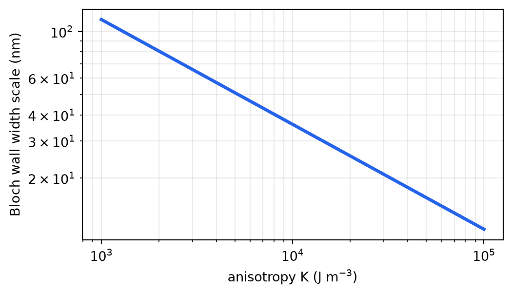
This chunk is deliberately small so the Quarto deck can render quickly while still proving that executable code works.
import numpy as np
import matplotlib.pyplot as plt

A = 1.3e-11
K = np.logspace(3, 5, 160)
delta_nm = np.sqrt(A / K) * 1e9

fig, ax = plt.subplots(figsize=(5.8, 3.2))
ax.loglog(K, delta_nm, color="#2563eb", lw=2.5)
ax.set_xlabel("anisotropy K (J m$^{-3}$)")
ax.set_ylabel("Bloch wall width scale (nm)")
ax.grid(True, which="both", alpha=0.25)
plt.show()
Figure 1: Domain-wall width decreases as anisotropy increases.