Slide 1

Introduction to atomistic and micromagnetic modeling

2026 IRM summer school

Slide 2

So far we have covered….
First principles theory + macroscopic experiments

•In theory:

•Fine-particle magnetism

•Domain states and their magnetic properties

•Magnetic mineralogy

•Material magnetic properties

•Magnetic anisotropy

•In the lab:

•Hystresis loop, backfield, FORC (VSM)

•NRM, TRM, IRM, ARM, etc (SQUID SRM)

•Temperature dependent remanence (MPMS measurements)

•X-T, AMS (Kappa bridge, MFK, magnon)

Slide 3

So far we have covered….
First principles theory + macroscopic experiments

•In the lab:

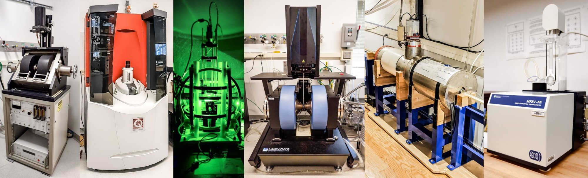
•X-T, AMS (Kappa bridge, MFK, magnon)

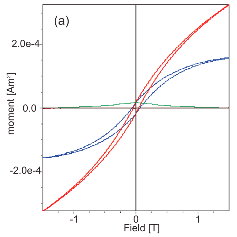
•Hystresis loop, backfield, FORC (VSM)

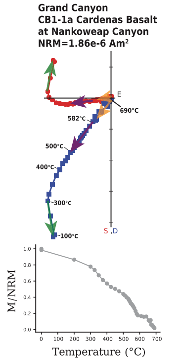
•NRM, TRM, IRM, ARM, etc (SQUID SRM)

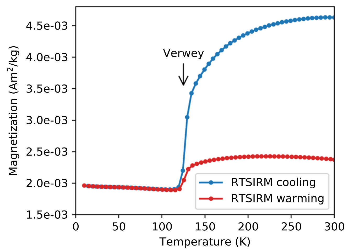
•Temperature dependent remanence (MPMS measurements)

Slide 4

So far we have covered….
First principles theory + macroscopic experiments

•In the lab:

•X-T, AMS (Kappa bridge, MFK, magnon)

•Hystresis loop, backfield, FORC (VSM)

•NRM, TRM, IRM, ARM, etc (SQUID SRM)

•Temperature dependent remanence (MPMS measurements)

Slide 5

So far we have covered….
First principles theory + macroscopic experiments

•In the lab:

•X-T, AMS (Kappa bridge, MFK, magnon)

•Hystresis loop, backfield, FORC (VSM)

•NRM, TRM, IRM, ARM, etc (SQUID SRM)

•Temperature dependent remanence (MPMS measurements)

Slide 6

So far we have covered….
First principles theory + macroscopic experiments

•In the lab:

•X-T, AMS (Kappa bridge, MFK, magnon)

•Hystresis loop, backfield, FORC (VSM)

•NRM, TRM, IRM, ARM, etc (SQUID SRM)

•Temperature dependent remanence (MPMS measurements)

Slide 7

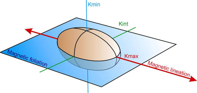
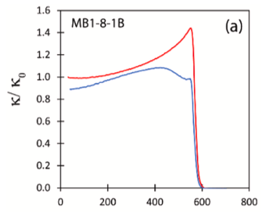
Results interpretation and experimental design depend on micromagnetic understanding

Slide 8

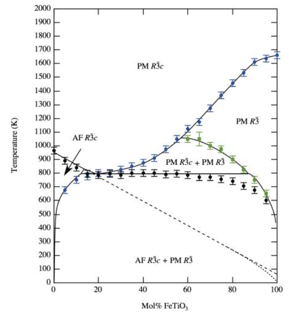
Computational material science

Length scale

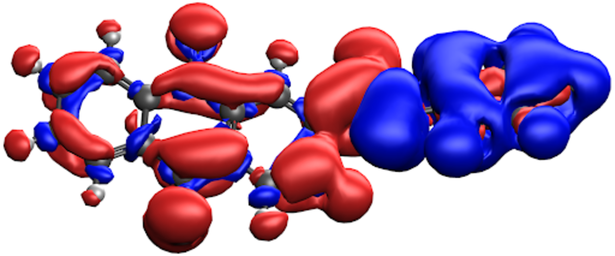
e.g. the Verwey transition

https://www.q-chem.com/explore/dft/cdft/

Ti-Fe oxide phase diagram

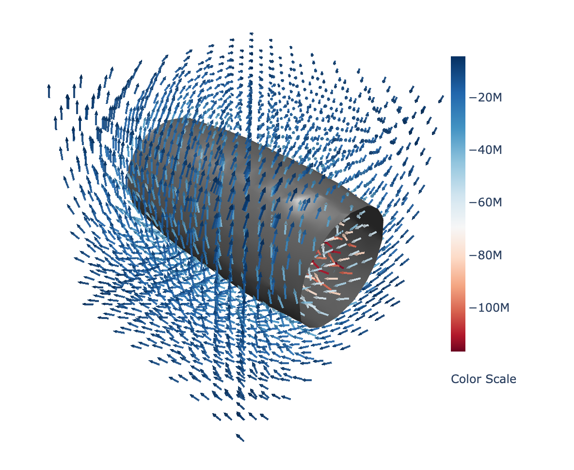
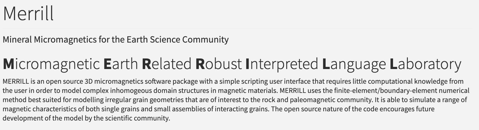
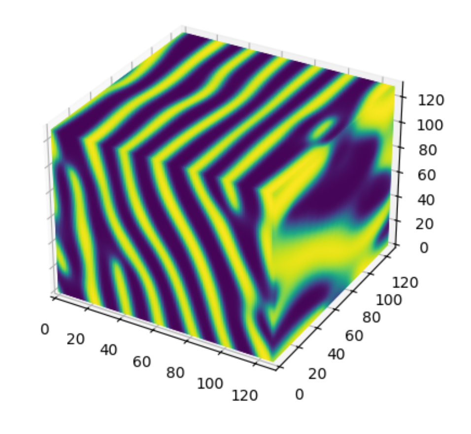
Micromagnetic modeling

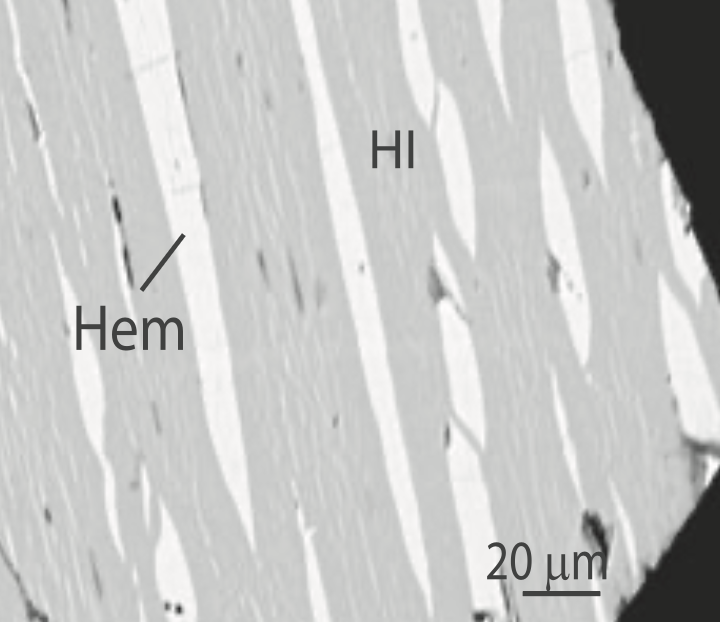
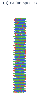
Exsolution modeling

Slide 9

Computational material science

Length scale

e.g. the Verwey transition

https://www.q-chem.com/explore/dft/cdft/

Ti-Fe oxide phase diagram

Micromagnetic modeling

Exsolution modeling

Slide 10

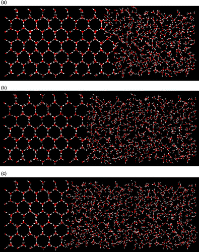
https://doi.org/10.1080/08927021003774287

water-ice

Slide 11

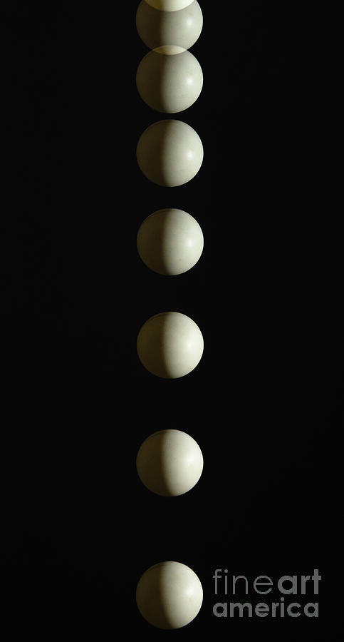
An introduction to Hamiltonian physics

Newtonian physics

$F=ma$

Tracking the force and velocity

Hamiltonian physics

$\begin{array}{rl}H=& E_{\mathrm{kinetic}}\\ & +E_{\mathrm{grav}}\\ & +E_{\mathrm{elastic}}\\ & +E_{\mathrm{heat}}\end{array}$

Tracking the system energy

Ideal magnetite: A and B cation sites

Ideal magnetite establishes the A–B site pattern

Inverse spinel: (Fe³⁺)_A[Fe²⁺Fe³⁺]_BO₄

A site
Fe³⁺ in an FeO₄ tetrahedron
One A cation per formula unit; its spin is antiparallel to the B sublattice.

B sites
Fe²⁺ + Fe³⁺ in FeO₆ octahedra
Two B cations per formula unit; their spins are parallel to one another.

The A- and B-site Fe³⁺ moments cancel ideally; B-site Fe²⁺ supplies the net moment.

Titanomagnetite: Ti substitutes into the magnetite lattice

Ti substitution changes chemistry and moment

TM25 example: (Fe³⁺)_A[Fe²⁺_1.25Fe³⁺_0.50Ti⁴⁺_0.25]_BO₄

Substitution
Fe³⁺(B) → Ti⁴⁺(B)
Ti enters an octahedral site that was occupied by Fe.

Charge balance
Fe³⁺ → Fe²⁺
Each Ti⁴⁺ adds one positive charge relative to Fe³⁺, so another Fe³⁺ is reduced to Fe²⁺.

Nonmagnetic Ti removes an Fe moment and changes the Fe²⁺/Fe³⁺ exchange network.

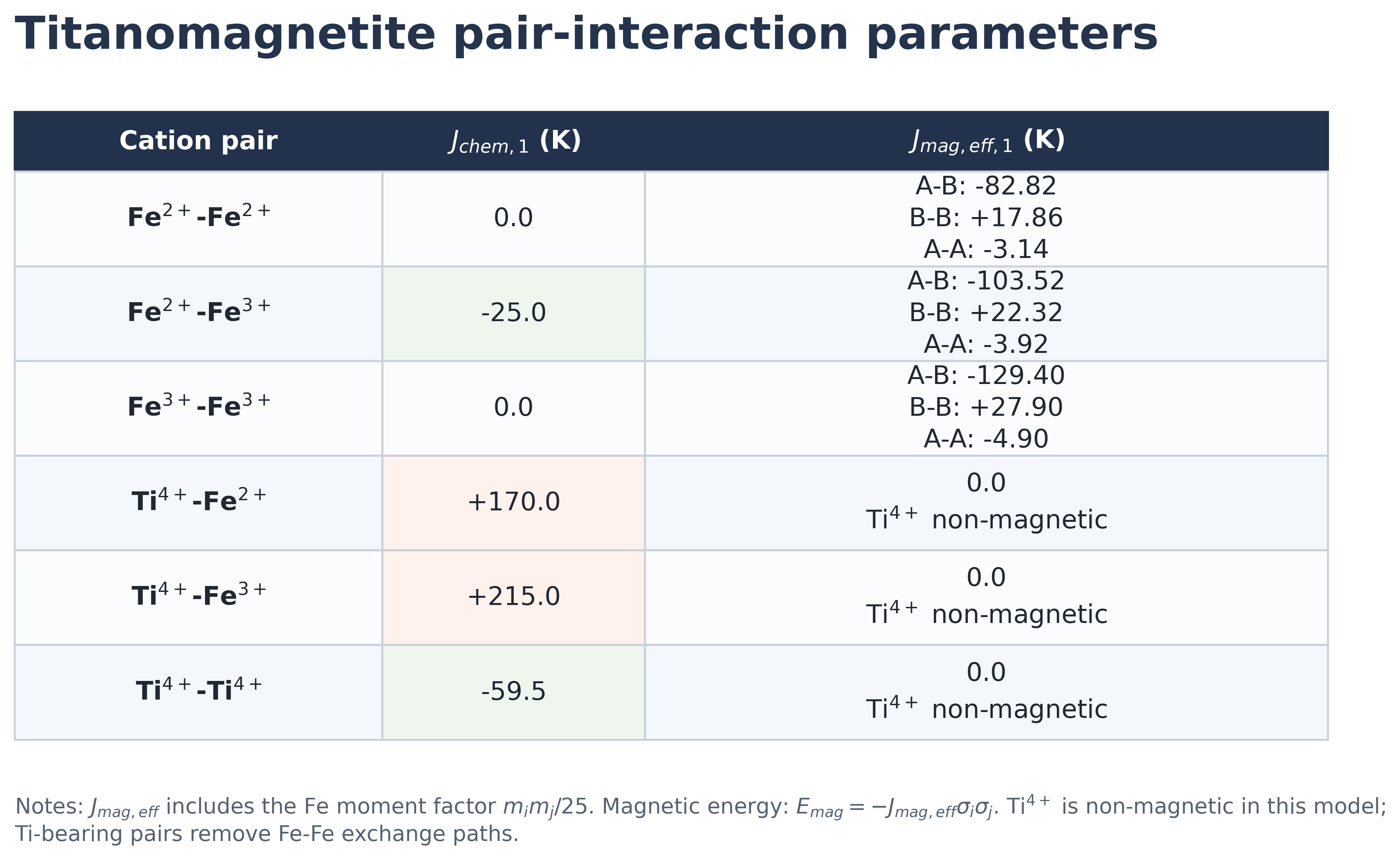
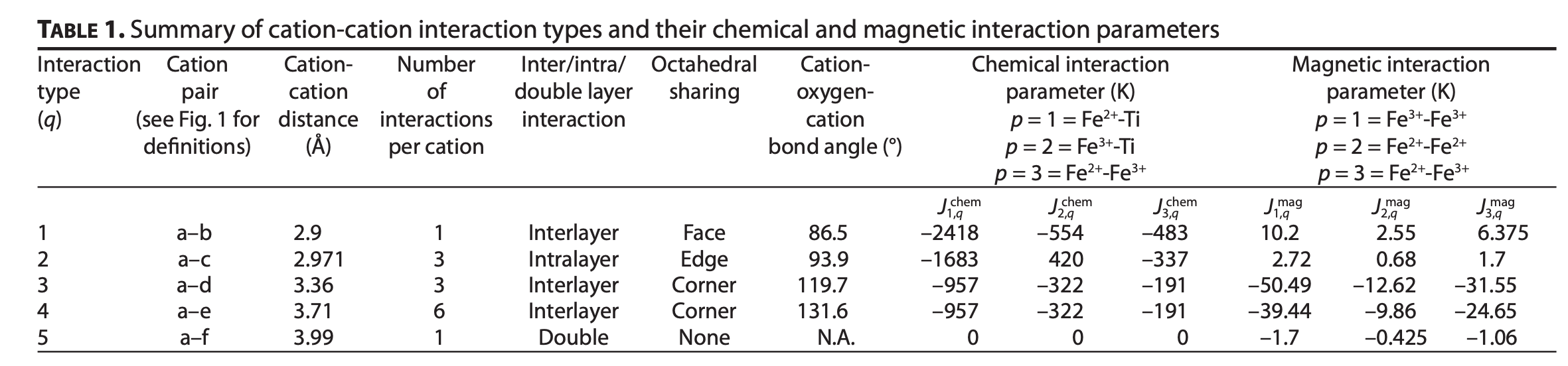
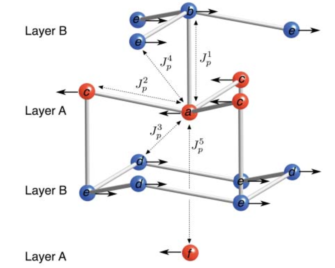
Titanomagnetite pair-interaction parameters

Slide 13

An introduction to the atomistic model
titanomagnetite energy model

$E_{\mathrm{total}}=E_{\mathrm{chem}}+E_{\mathrm{mag}}.$

The chemical energy asks which cation arrangements are favorable.

$E_{\mathrm{chem}}=E_{\mathrm{site}}+{\sum }_p{J}_p^{(\mathrm{chem})}{N}_p,$

where $N_{\mathrm{pair}}$ is the number of neighbor pairs of a particular type. Positive interaction terms make those neighbor pairs energetically costly; negative terms make them favorable.

The magnetic energy asks how neighboring Fe spins prefer to align.

$E_{\mathrm{mag}}=-{\sum }_{ij}{J}_{ij}^{(\mathrm{mag})}{\sigma }_i{\sigma }_j,$

where ${\sigma }_i$ is the spin sign on Fe site $i$. This is simpler than real titanomagnetite magnetism, but it captures the key teaching idea: the Fe spin network depends on which cations occupy which sites.

Slide 14

An introduction to the atomistic model
titanomagnetite energy model

$E_{\mathrm{total}}=E_{\mathrm{chem}}+E_{\mathrm{mag}}.$

The chemical energy asks which cation arrangements are favorable.

$E_{\mathrm{chem}}=E_{\mathrm{site}}+{\sum }_p{J}_p^{(\mathrm{chem})}{N}_p,$

where $N_{\mathrm{pair}}$ is the number of neighbor pairs of a particular type. Positive interaction terms make those neighbor pairs energetically costly; negative terms make them favorable.

The magnetic energy asks how neighboring Fe spins prefer to align.

$E_{\mathrm{mag}}=-{\sum }_{ij}{J}_{ij}^{(\mathrm{mag})}{\sigma }_i{\sigma }_j,$

where ${\sigma }_i$ is the spin sign on Fe site $i$. This is simpler than real titanomagnetite magnetism, but it captures the key teaching idea: the Fe spin network depends on which cations occupy which sites.

TM30 at 160 K and 700 K

TM30 at 160 K and 700 K: spin order is more temperature-sensitive

Same 6 × 6 × 1 cell, TM30 composition, random starting state, 60,000 trials, Hamiltonian, and seed; only temperature changes.

160 K

700 K

Ti B-site order 0.86 · pair order 0.91 · global order 0.67

Ti B-site order 0.79 · pair order 0.53 · global order 0.025

Heating largely randomizes the Fe-spin network before it erases Ti’s preference for B sites.

Slide 15

An introduction to the atomistic model
titanomagnetite energy model

$E_{\mathrm{total}}=E_{\mathrm{chem}}+E_{\mathrm{mag}}.$

The chemical energy asks which cation arrangements are favorable.

$E_{\mathrm{chem}}=E_{\mathrm{site}}+{\sum }_p{J}_p^{(\mathrm{chem})}{N}_p,$

where $N_{\mathrm{pair}}$ is the number of neighbor pairs of a particular type. Positive interaction terms make those neighbor pairs energetically costly; negative terms make them favorable.

The magnetic energy asks how neighboring Fe spins prefer to align.

$E_{\mathrm{mag}}=-{\sum }_{ij}{J}_{ij}^{(\mathrm{mag})}{\sigma }_i{\sigma }_j,$

where ${\sigma }_i$ is the spin sign on Fe site $i$. This is simpler than real titanomagnetite magnetism, but it captures the key teaching idea: the Fe spin network depends on which cations occupy which sites.

Read the orange and gray curves as the central thermodynamic estimate. The binodal encloses the spinodal at every sampled temperature, the endmember mixing entropies return to zero, and the branches close symmetrically for the stated Akimoto cation model. These checks support the topology of a magnetite-ulvospinel miscibility gap.

Do not present the absolute top of the solvus as precisely known. Propagating the quoted Lilova mixing-enthalpy uncertainty through this simplified free-energy model moves the modeled consolute temperature from roughly 150 to 660 degrees Celsius. The central curve closes near 400 degrees Celsius. It is a useful teaching estimate, not a high-precision experimental boundary.

The blue line is still less formal. It is an operational B-site spin-order threshold from a finite 8 by 8 by 4 simulation cell, five random seeds, and a 50 K temperature grid. It is included to compare atomistic ordering trends with the thermodynamic diagram, not as an equilibrium phase boundary.

Sublattice competition produces Q- and P-type curves

Sublattice competition produces Q- and P-type curves

Start with the exact ionic limit for inverse-spinel magnetite: the A-site Fe3+ contribution is 5 Bohr magnetons antiparallel to 9 on the B sublattice, leaving 4 per formula unit. That difference, not the sum, is the spontaneous moment.

Use TM60 here as the representative P-type case. The plotted curves are now a self-consistent solution of two coupled Brillouin equations, not independent empirical decay functions. The effective molecular field acting on each sublattice is produced by the other sublattice. In the TM60 reduction, the A contribution weakens slightly faster at low temperature; because the measured ferrimagnetic moment is the difference (M_B-M_A), that loss of opposing A moment first makes the net moment rise by about 5%. The maximum occurs near (T/T_C=0.42), where reduced temperature uses kelvin. With (T_C) about 436 K for TM60, this places the maximum near 183 K, or minus 90 degrees Celsius. Both sublattices then collapse toward the Curie temperature.

For teaching clarity, the plot reduces the calculation to two effective A and B sublattices. Stephenson’s fuller titanomagnetite treatment resolves four molecular fields: Fe2+ and Fe3+ on both A and B sites, with the dominant A-B interactions coupled self-consistently. The present coupling asymmetry is therefore a topology-constrained lecture calibration, not a unique inversion for every microscopic exchange constant. A research upgrade should fit those four ion/site fields to sublattice-sensitive thermomagnetic or neutron data.

Hematite’s weak moment comes from canted antiferromagnetism

Hematite’s weak moment comes from canted antiferromagnetism

Begin with the crystal rather than the magnetic equation. Hematite has the corundum structure, space group R-3c. The gray oxygen ions make a distorted close-packed framework, and Fe3+ occupies two-thirds of the available octahedral sites. The view repeats the conventional cell twice along each basal translation so that several Fe ions are visible in every plane. The coordination guides around the two highlighted iron ions make the FeO6 environment visible.

The red and blue labels identify alternating cation layers A and B. They are not the tetrahedral A and octahedral B sites used for spinel magnetite; chemically, both hematite layer families contain octahedrally coordinated Fe3+. Each Harrison layer is a buckled sheet that resolves into two closely spaced Fe planes. The animation therefore labels three complete cation layers A-B-A, while the individual plane moments follow plus-plus-minus-minus-plus-plus. The brackets group the two planes belonging to each layer. Their close separation is only the projection along c; lateral offsets determine the full three-dimensional Fe-Fe distances. Within each layer the moments are nearly parallel, while adjacent A and B layers are antiparallel and largely compensate.

Use the room-temperature button first. Above the Morin transition, the dominant Fe moments lie in the basal plane. If the two sublattice vectors were exactly antiparallel, their sum would be zero. The Dzyaloshinskii-Moriya interaction rotates them by a tiny common sense: the large plus and minus components still cancel, but the two small transverse components point the same way and add. In the animation the red and blue display vectors are defined once, and the gold vector is calculated directly from their component-by-component sum, so its direction and relative length are exact for the exaggerated drawing. The gold arrow is therefore a weak ferromagnetic moment, not an uncompensated full Fe3+ moment. The drawing exaggerates the canting enormously. Each sublattice is tilted by about 0.065 degrees, giving roughly 0.13 degrees between the real spin pair and exact antiparallel alignment.

Then toggle below the Morin transition. The lattice does not reconstruct. Instead, the preferred spin direction rotates toward the c axis and the weak basal-plane moment is suppressed. This is the structural and magnetic starting point for the hemo-ilmenite model that follows: chemical ordering and lamellae modify how these Fe-rich magnetic layers couple.

Sources for the teaching schematic and magnetic convention: Roberts et al. (2021), Journal of Geophysical Research: Solid Earth, doi:10.1029/2021JB023027; Jiang et al. (2014), Geochemistry, Geophysics, Geosystems, doi:10.1002/2014GC005377. Ambient hematite lattice parameters are represented schematically; the purpose is to show coordination, layer geometry, and spin directions rather than refine a crystallographic structure.

Slide 16

Hemo-ilmenite lamellar magnetism

Harrison, 2006

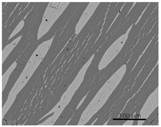
McEnroe et al., 2007

Slide 17

Hemo-ilmenite lamellar magnetism

Harrison, 2006

Slide 18

Hemo-ilmenite lamellar magnetism

Harrison, 2006

Slide 19

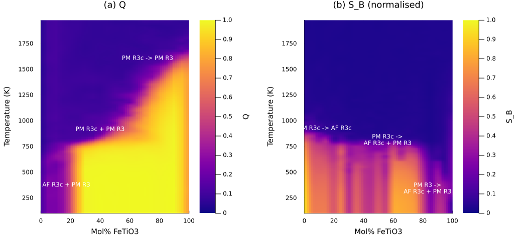
Hemo-ilmenite lamellar magnetism

Harrison, 2006

Slide 20

Hemo-ilmenite lamellar magnetism

Harrison, 2006

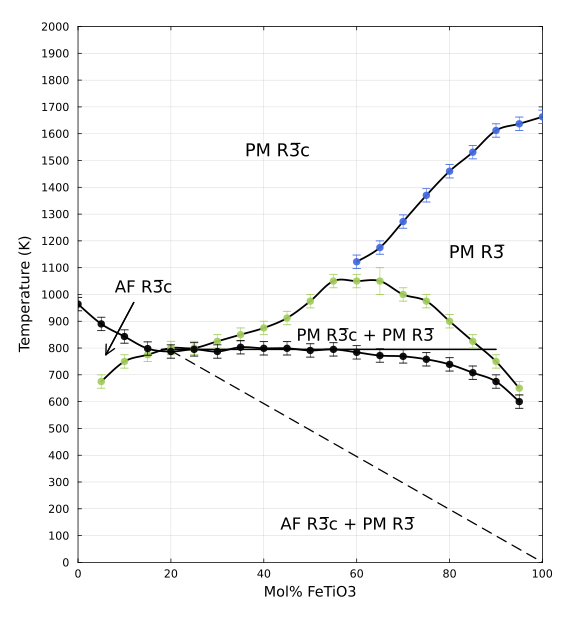
Hematite

Neel temperature

Slide 21

Mesoscale Modeling
previous theory and modeling

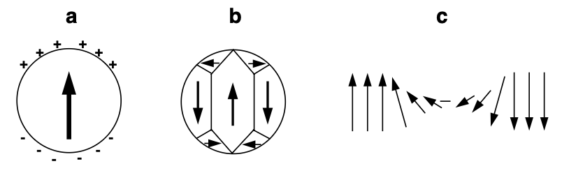
Butler, 1992

Slide 22

Mesoscale Modeling
previous theory and modeling

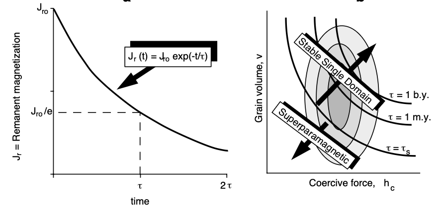
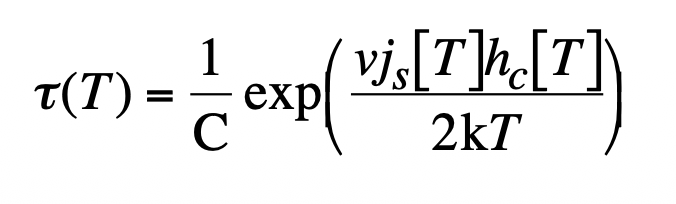
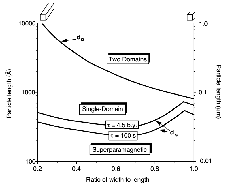
Butler, 1992; Néel 1955

Slide 23

Natural magnetic grains in rocks

5 X

10 X

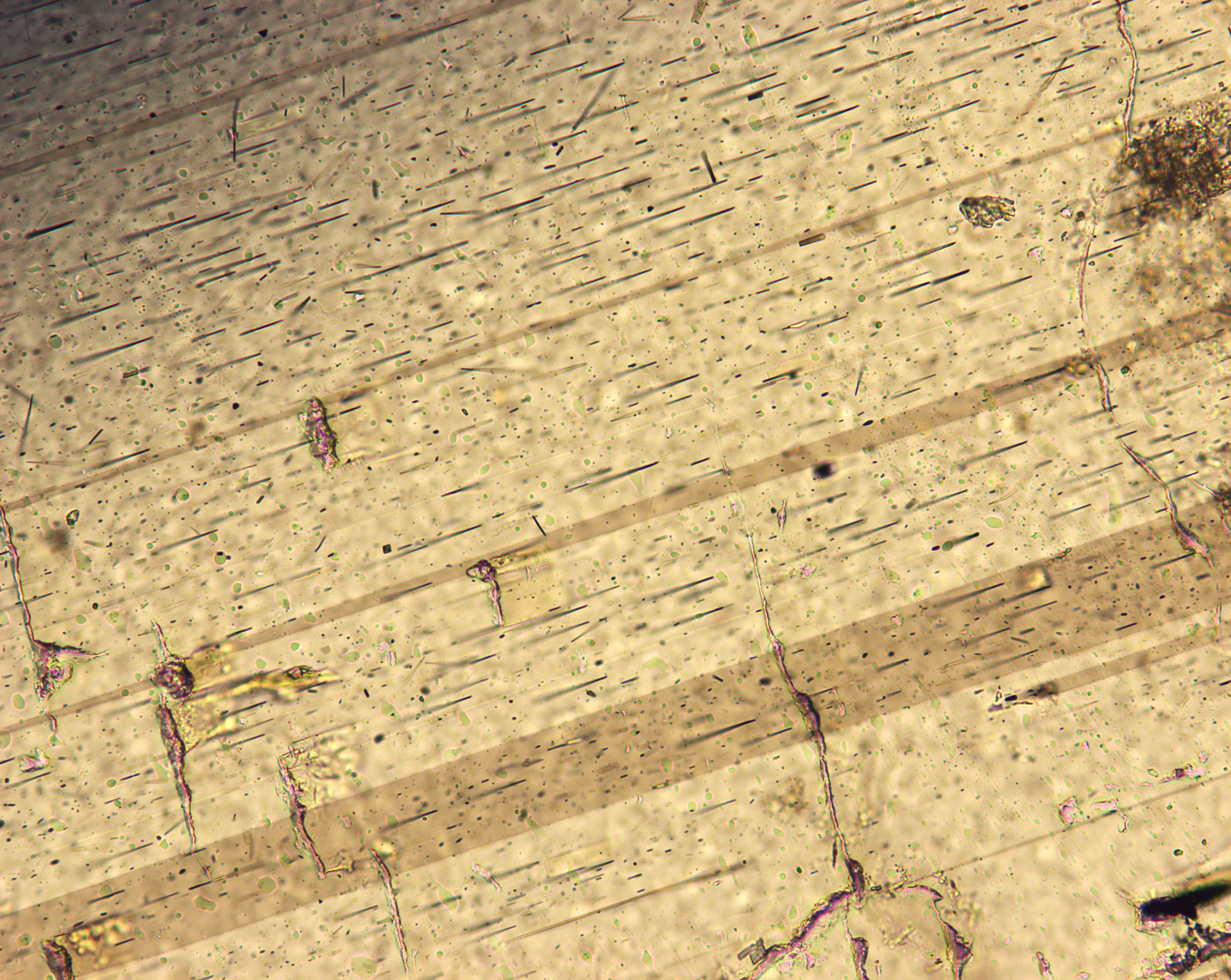
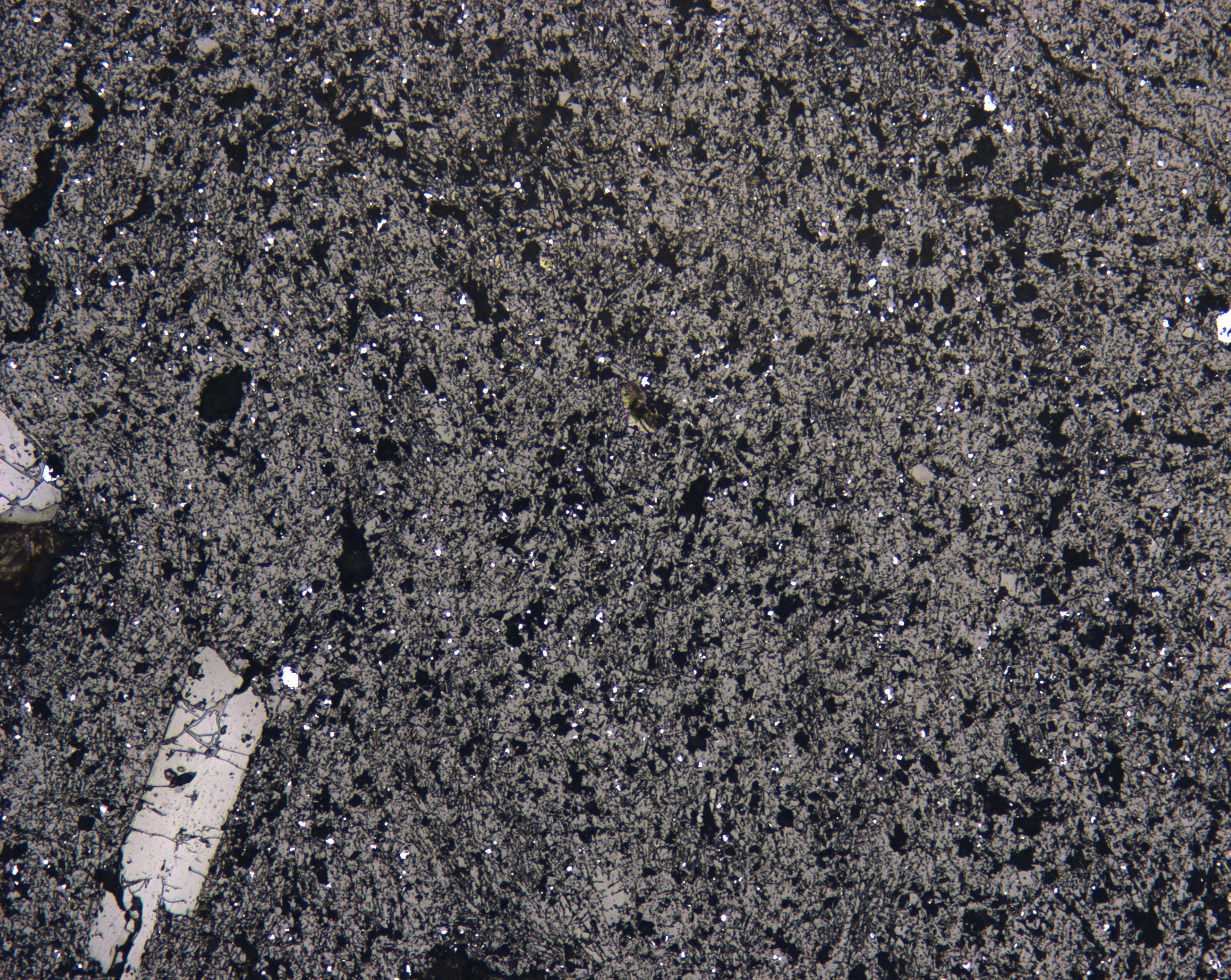
Berkeley Hills volcanic rock

Minnesota plagioclase in intrusive rock

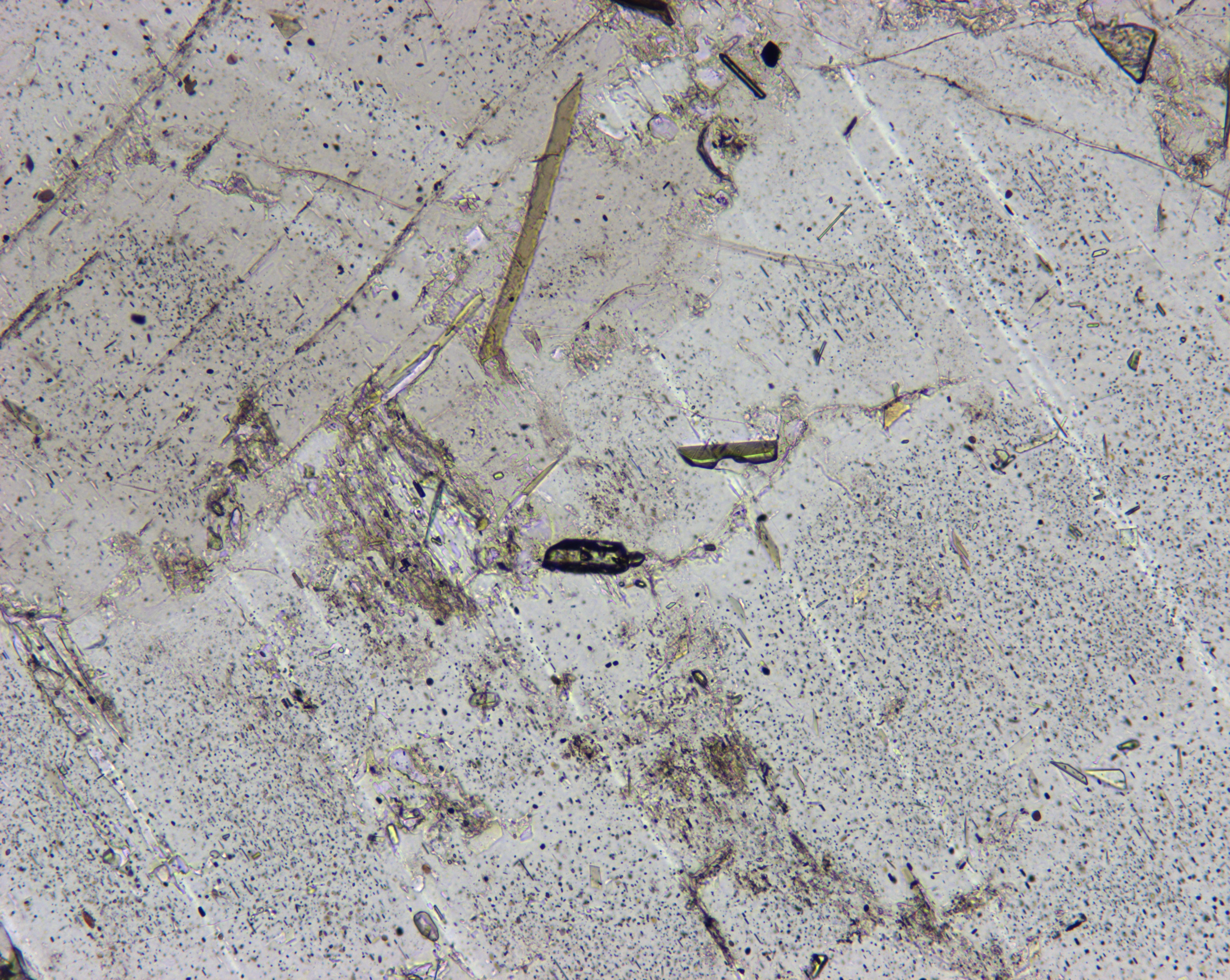
Metamorphosed anorthosite from Quebec

10 X

Slide 24

Natural magnetic grains in rocks

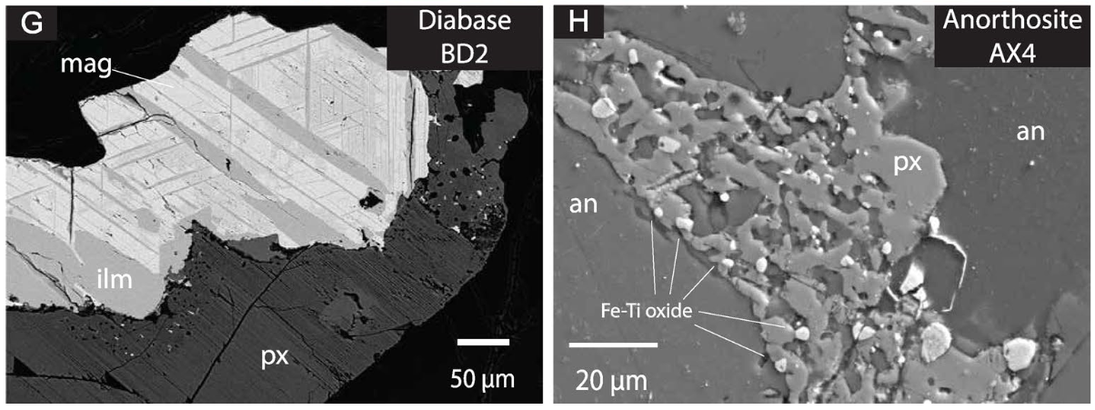
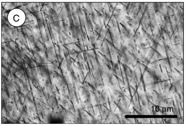
Feinberg et al., 2006

Zhang et al., 2021

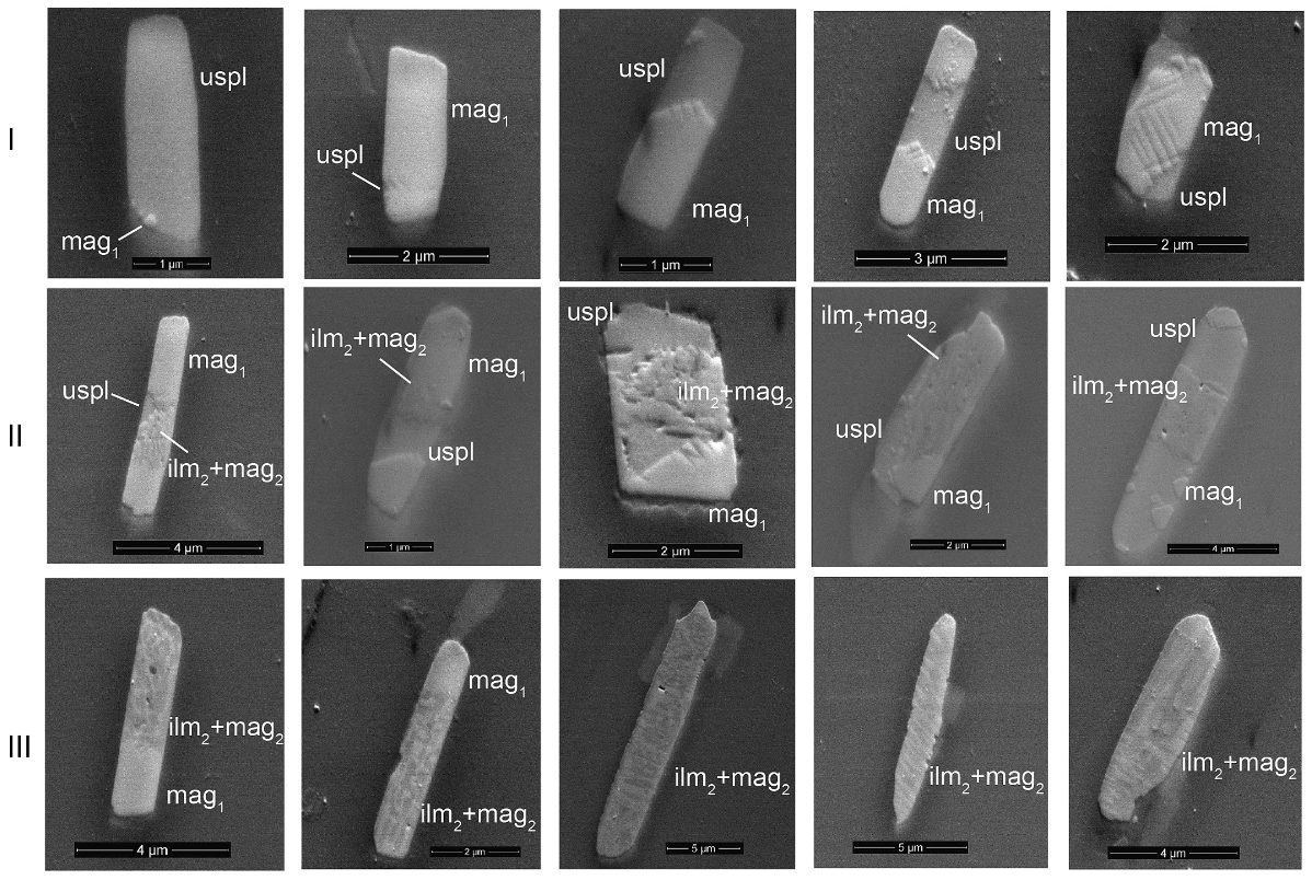
Bian et al., 2025

Slide 25

Natural magnetic grains in rocks

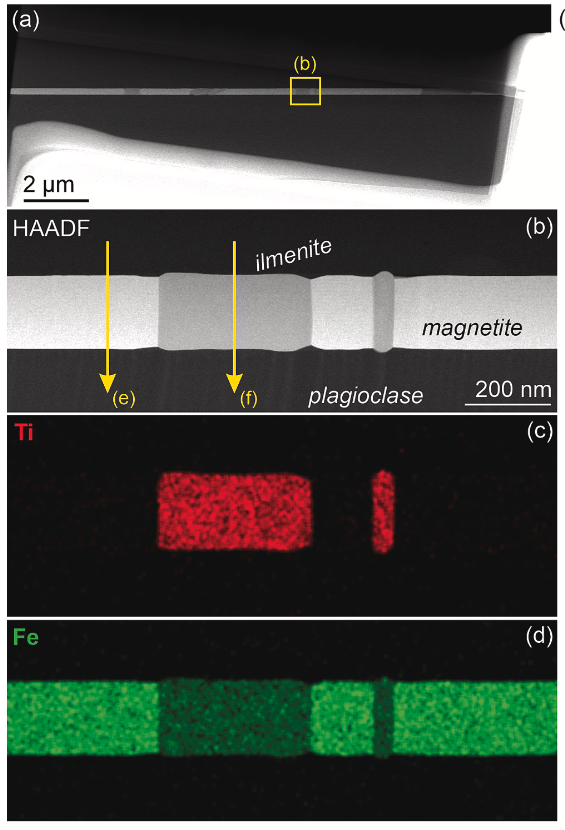
Bian et al., 2025

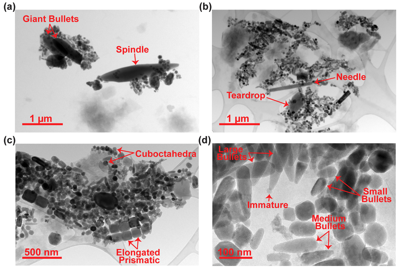
Wagner et al., 2021

Slide 26

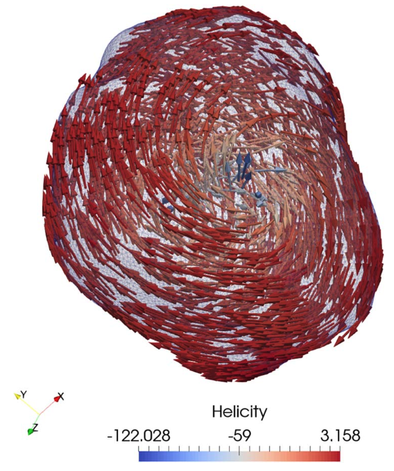
Wyn Williams

Karl Fabian

Lesleis Nagy

Slide 27

Difference between materials research and rock magnetism research

Materials research

-Regular geometries

-Homogeneous composition

-Very short timescales

-Landau-Lifshitz-Gilbert equation

-Finite difference modeling

Slide 28

Difference between materials research and rock magnetism research

Rock magnetism research

-Irregular geometries

-Homogeneous/heterogeneous composition

-Large range of timescales

-Local energy minima (LEM)

-Finite element modeling

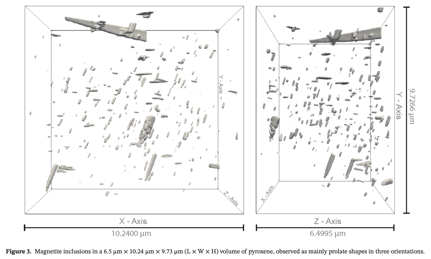
Nikolaisen et al., 2020

Slide 29

FEM micromagnetic modeling

•Represent realistic grain geometry with small tetrahedron mesh

•Each tetrahedron represents a small chunk of atoms

Approximate micromagnetic behaviors

Anisotropy energy

Exchange energy

Demagnetizing energy

External field energy (Zeeman energy)

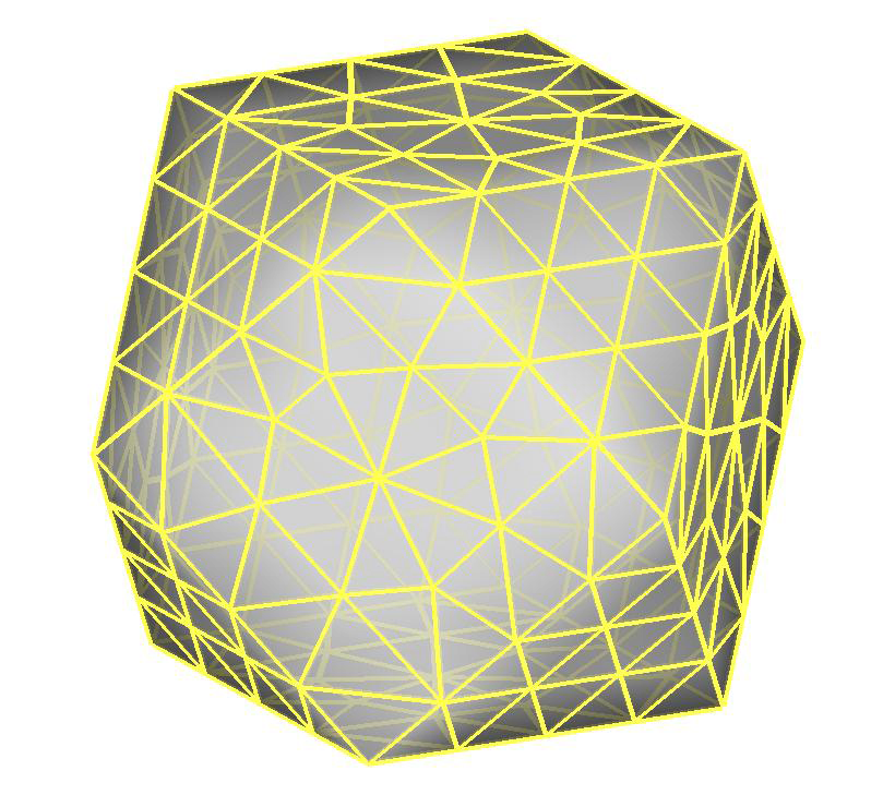
Hamiltonian physics is a way of describing motion and stability using energy, and in micromagnetics it helps us understand how tiny magnetic moments choose their directions by balancing different energy costs and rewards.

Slide 30

Magnetocrystalline:cubic

The Magnetic Energy Components

Micromagnetic Theory

Modified slide from Wyn Williams

${\alpha }_1$, ${\alpha }_2$, ${\alpha }_3$ are the direction cosines

of the magnetization vector

and $K_1$ and $K_2$ are the (temperature-dependent)

crystalline anisotropy constants

$E_{\mathrm{cub}}=\sum _{x,y,z}\left[K_1\left({\alpha }_1^2{\alpha }_2^2+{\alpha }_2^2{\alpha }_3^2+{\alpha }_3^2{\alpha }_1^2\right)+K_2{\alpha }_1^2{\alpha }_2^2{\alpha }_3^2\right]$

Example shown: M ∥ [111]. Rotating the collective ferrimagnetic moment changes α₁, α₂, α₃—and therefore E_cub—even though the cation lattice is unchanged.

Slide 31

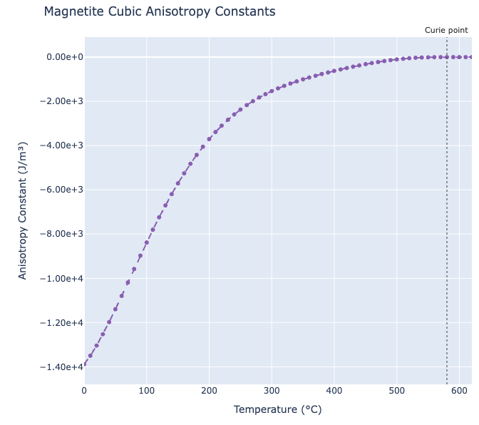
Magnetocrystalline:cubic

The Magnetic Energy Components

Micromagnetic Theory

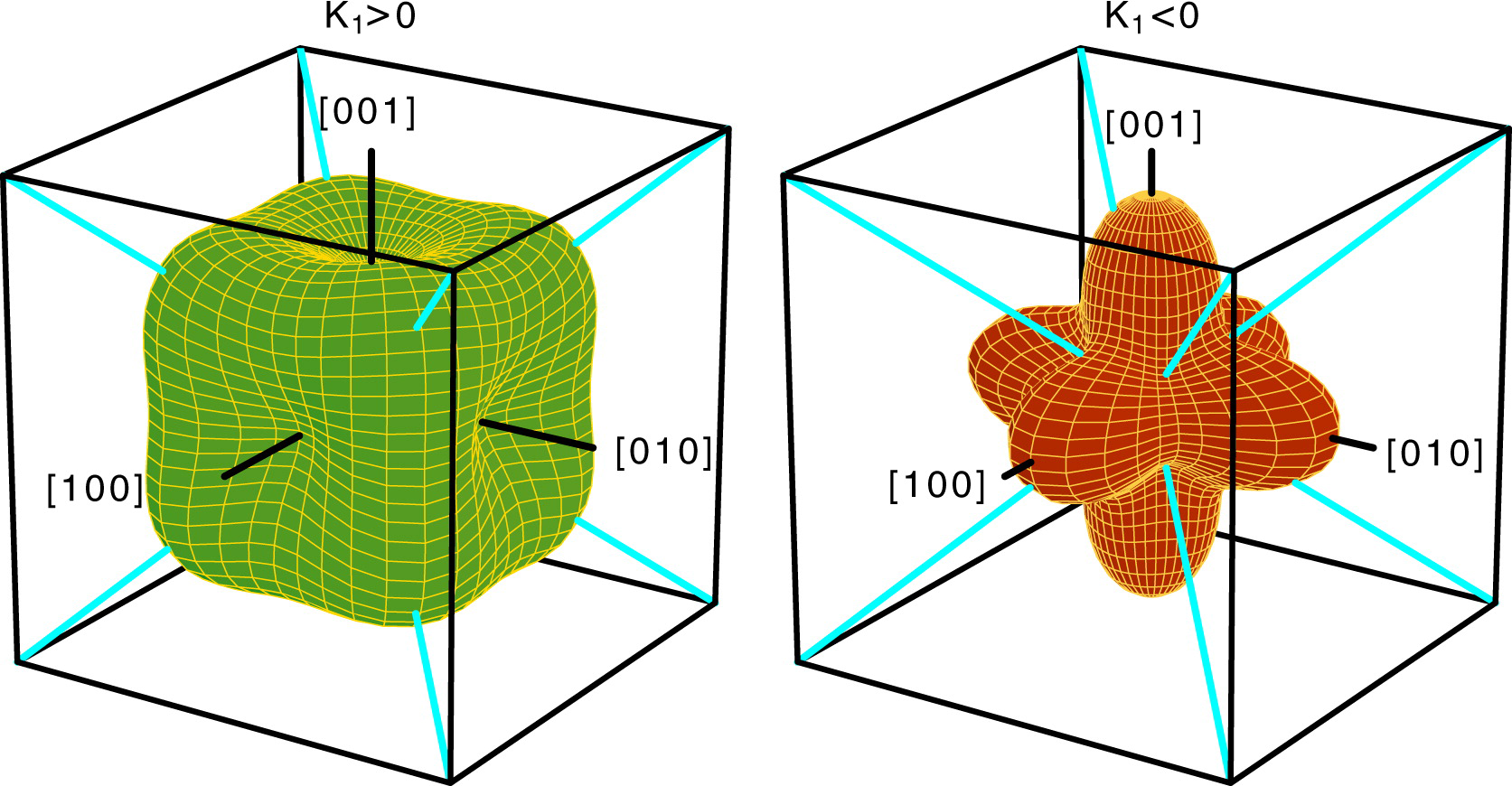
${\alpha }_1$, ${\alpha }_2$, ${\alpha }_3$ are the direction cosines

of the magnetization vector

and $K_1$ and $K_2$ are the (temperature-dependent)

crystalline anisotropy constants

$E_{\mathrm{cub}}=\sum _{x,y,z}\left[K_1\left({\alpha }_1^2{\alpha }_2^2+{\alpha }_2^2{\alpha }_3^2+{\alpha }_3^2{\alpha }_1^2\right)+K_2{\alpha }_1^2{\alpha }_2^2{\alpha }_3^2\right]$

Modified slide from Wyn Williams

Slide 32

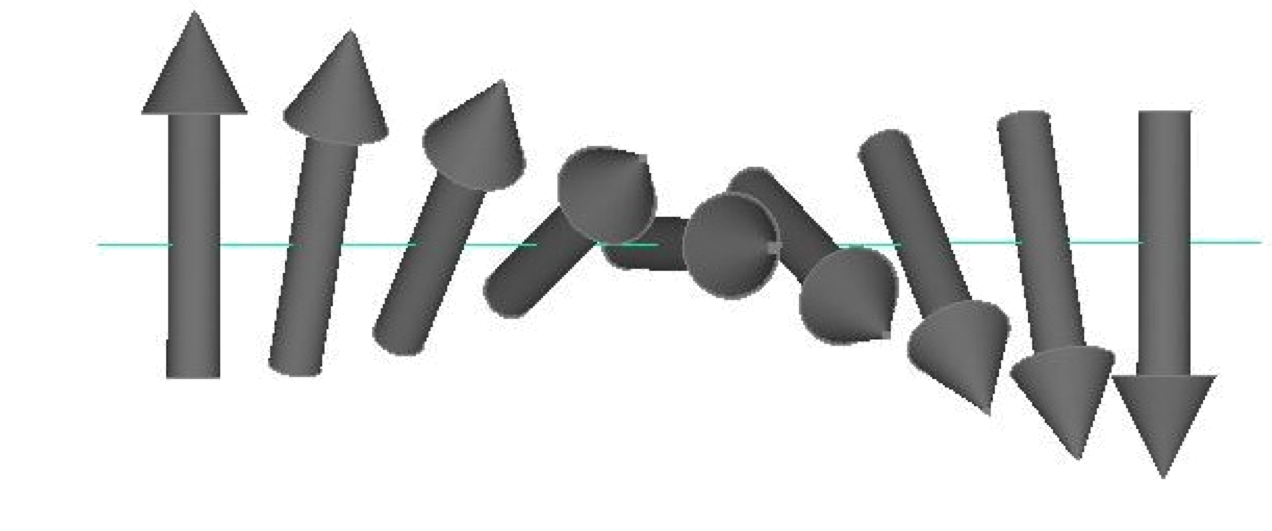
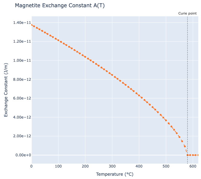
Exchange

The Magnetic Energy Components

Micromagnetic Theory

${\sum }_{x,y,z}\left[A_E{\left(\nabla \mathbf{m}\right)}^2\right]$

$\mathbf{m}$ is the local magnetization direction

$\nabla \mathbf{m}$ means how rapidly changes in space.

$A_E$: temperature-dependent exchange constant

$\nabla \mathbf{m}=\left(\frac{\partial m_x}{\partial x},\frac{\partial m_x}{\partial y},\frac{\partial m_x}{\partial z}\right)$

Modified slide from Wyn Williams

Slide 33

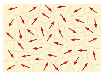
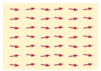
External Field (Zeeman energy)

The Magnetic Energy Components

Micromagnetic Theory

$-{\mu }_0{M}_S{\sum }_{x,y,z}\left[\mathbf{m}\cdot {\mathbf{H}}_e\right]$

$M_S$ is the (temperature-dependent)

saturation (intrinsic) magnetization

${\mathbf{H}}_e$

No field

Slide from Wyn Williams

Slide 34

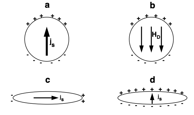
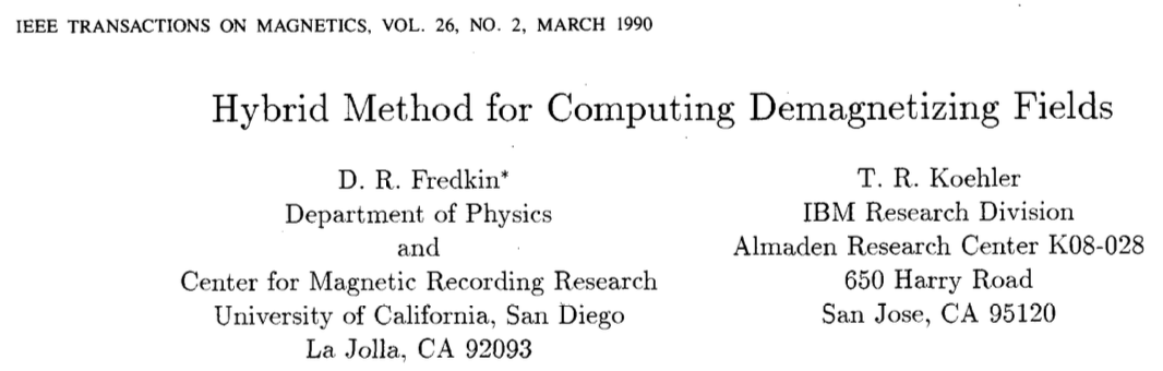
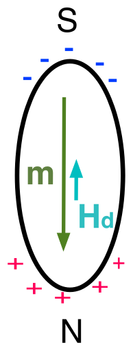
Demagnetizing energy (Stray field)

The Magnetic Energy Components

Micromagnetic Theory

$\varnothing$ is the magnetic scalar potential and must be defined in all space.

${\nabla }^2\varnothing =\nabla \cdot \mathbf{m}$

${\mathbf{H}}_{\mathrm{demag}}=\nabla \varnothing$

$\varnothing (\infty )=0$

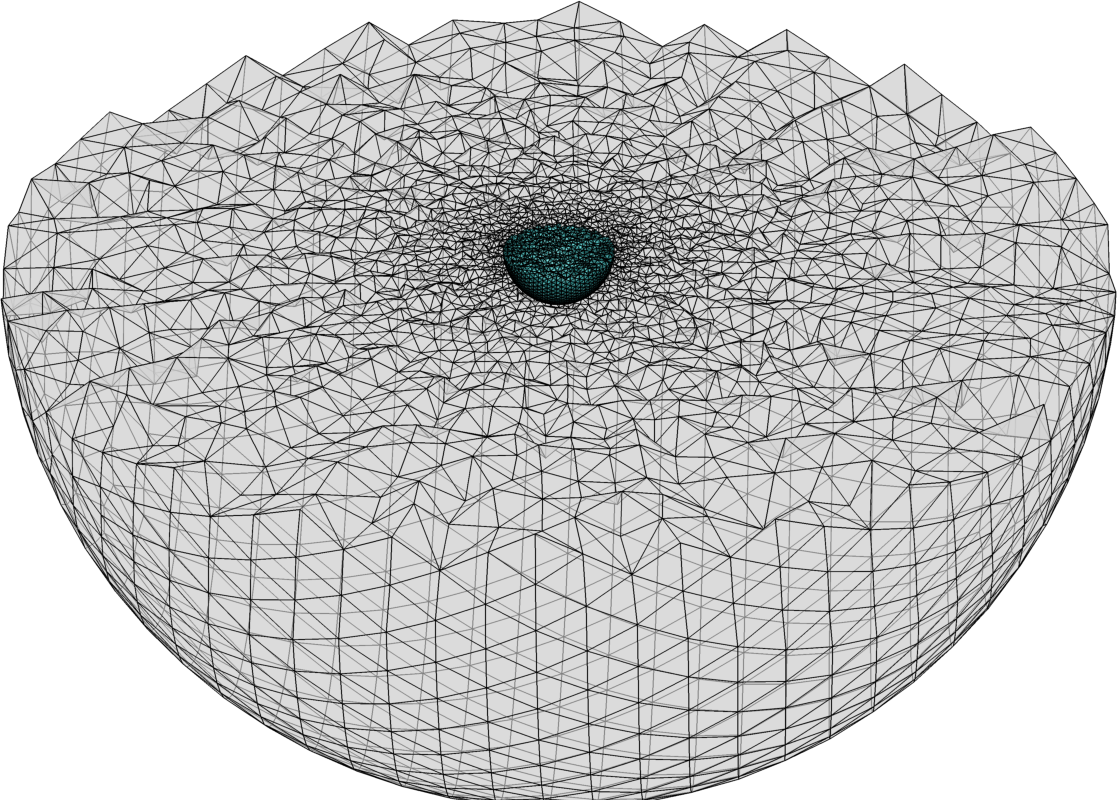
Modified slide from Wyn Williams

Slide 35

Demagnetizing energy (Stray field)

The Magnetic Energy Components

Micromagnetic Theory

$\varnothing$ is the magnetic scalar potential and must be defined in all space.

${\nabla }^2\varnothing =\nabla \cdot \mathbf{m}$

${\mathbf{H}}_{\mathrm{demag}}=-\nabla \varnothing$

${\mathbf{H}}_d=-\frac{\mathbf{m}}{3}$

$\varnothing (\infty )=0$

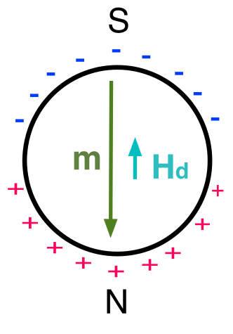
Slide from Wyn Williams

Slide 36

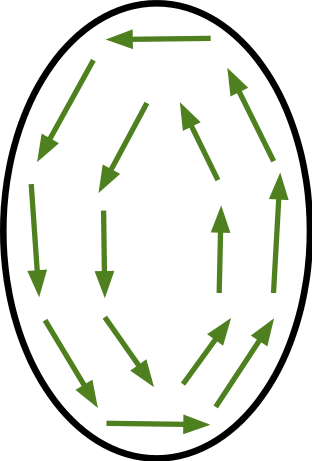
Demagnetizing energy (Stray field)

The Magnetic Energy Components

Micromagnetic Theory

$\varnothing$ is the magnetic scalar potential

${\nabla }^2\varnothing =\nabla \cdot \mathbf{m}$

${\mathbf{H}}_{\mathrm{demag}}=-\nabla \varnothing$

$\varnothing (\infty )=0$

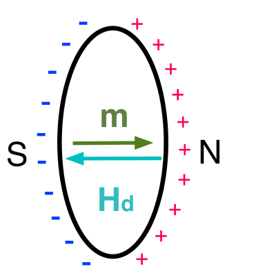
Slide from Wyn Williams

${\sigma }_m=\mathbf{M}\cdot \mathbf{n}$

E_demag = −½ μ₀ ∫_V M · H_d dV

Stray fields store energy wherever they extend—in and around the grain.

Because H_d opposes M, the minus sign gives a positive energy cost.

Reducing surface poles and closing magnetic flux lowers this energy.

Slide 37

The Magnetic Energy Components

Micromagnetic Theory

$E_{\mathrm{total}}=E_{\mathrm{exchange}}+E_{\mathrm{anisotropy}}+E_{\mathrm{demag}}+E_{\mathrm{Zeeman}}$

Slide 38

The Magnetic Energy Components

Micromagnetic Theory

$E_{\mathrm{total}}=E_{\mathrm{exchange}}+E_{\mathrm{anisotropy}}+E_{\mathrm{demag}}+E_{\mathrm{Zeeman}}$

Slide 39

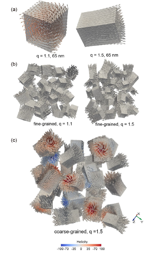
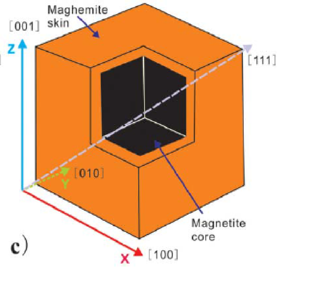
Micromagnetic Modeling

Single particles or assemblages

Variable composition

Oxidation: core-shell

Realistic natural particle morphologies

Focused-ion-beam nanotomography

Magnetic particle in obsidian

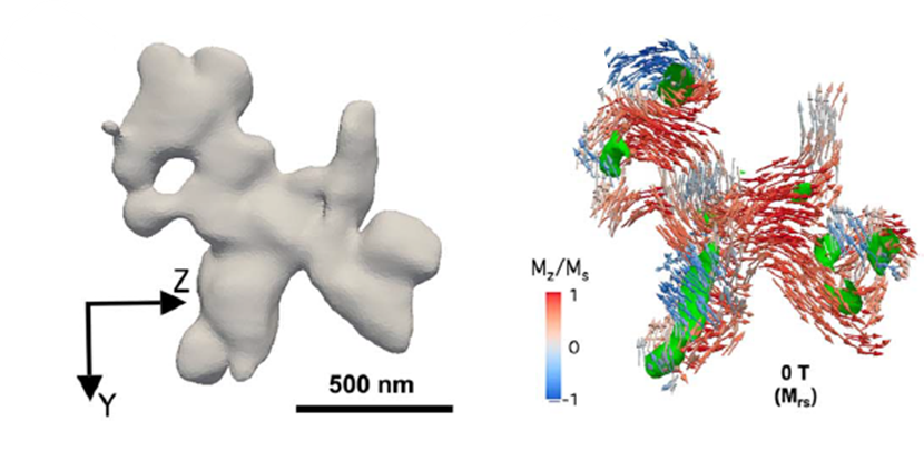
Ge et al. 2014

Bai et al. 2021

Lascu et al. 2018

Simulate

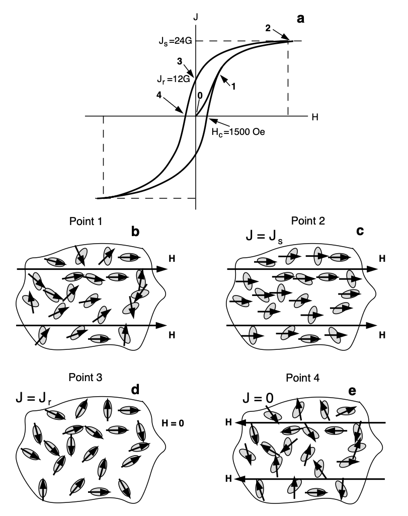
•Hysteresis

•Remanence curves

•FORC diagrams

•Relaxation times

Slide from Bruce Moskowitz

Slide 40

Micromagnetic application
revealing possible magnetization configurations

Slide 41

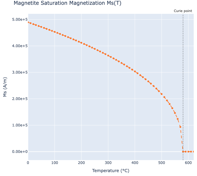
Micromagnetic application
simulate temperature-dependent experiments

$E_{\mathrm{total}}=E_{\mathrm{exchange}}+E_{\mathrm{anisotropy}}+E_{\mathrm{demag}}+E_{\mathrm{Zeeman}}$

Slide 42

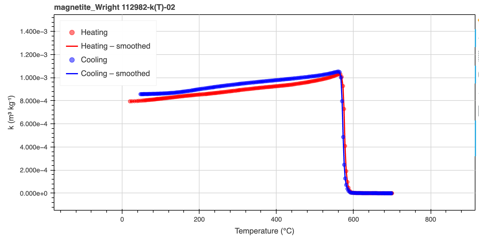
Micromagnetic application
simulate temperature-dependent magnetic susceptibility

$\chi \sim \frac{dm}{dB}$

Small single-domain hysteresis

Micromagnetic application
30 nm single-domain sphere: abrupt coherent switching

Slide 43

Micromagnetic application
simulate hysteresis experiments

Slide 44

Micromagnetic application
investigate the transition between states

$E_{\mathrm{saddle}}={\max }_k\left(E_k\right)$

$\Delta E_{ij}=E_{\mathrm{saddle}}-E_i$

$k_{ij}={\tau }_0^{-1}\exp \left(-\frac{\Delta E_{ij}}{k_{B}T}\right)$

${\tau }_{ij}=k_{ij}^{-1}={\tau }_0\exp \left(\frac{\Delta E_{ij}}{k_{B}T}\right)$

NEB relaxes the path sideways

Micromagnetic application
NEB finds the pass by relaxing each image perpendicular to the path

This is a three-dimensional rendering of the two-coordinate teaching example in Figure 4 of Nagy et al. The horizontal coordinates are the spherical angles theta and phi of a uniform magnetization vector, while the vertical coordinate is magnetic energy. The prolate ellipsoid’s long axis is [100]. Shape anisotropy makes plus and minus [100] the two endpoint minima. The negative cubic anisotropy of magnetite lowers the route through the [011]-type direction, so the curved path passes near theta equals pi over two and phi equals pi over four.

Begin with the red path. It is the direct angular interpolation at phi equals pi over two and crosses the higher [010]-type ridge. The dark-outlined white band contains discrete NEB images. The endpoints remain fixed. A small initial perturbation selects the lower of the two symmetry-related routes around the ridge.

Focus on the highlighted red image. The cyan arrow is the local path tangent. The gray arrow is the full downhill force, minus the energy gradient. NEB removes the component of this physical force parallel to the path and retains only the thick red perpendicular component. That retained component changes the shape of the path rather than allowing all images to slide into the endpoint minima. Its displayed length is exaggerated by a factor of 1.75 so that the update direction remains unmistakable to the audience; its direction is unchanged. The artificial spring force acts only parallel to the path, where it maintains useful spacing between images.

At convergence, the red perpendicular arrow shrinks toward zero. The gray energy-gradient arrow need not vanish except at a true stationary point such as the saddle: along the rest of the minimum-energy path, the remaining gradient is parallel to the path. Emphasize that perpendicular means perpendicular in configuration space, not normal to the rendered three-dimensional surface. The energy axis has been added only to make the barrier visible.

[Sources] - Nagy, L., Williams, W., Muxworthy, A. R., Fabian, K., Almeida, T. P., Ó Conbhuí, P., and Shcherbakov, V. P. (2017). Stability of equidimensional pseudo-single-domain magnetite over billion-year timescales. Proceedings of the National Academy of Sciences, 114, 10356-10360. https://doi.org/10.1073/pnas.1708344114. Figure 4 and accompanying description. - Henkelman, G., and Jónsson, H. (2000). Improved tangent estimate in the nudged elastic band method for finding minimum energy paths and saddle points. Journal of Chemical Physics, 113, 9978-9985. https://doi.org/10.1063/1.1323224. [/Sources]

Slide 45

Micromagnetic application
investigate the transition between states

Slide 46

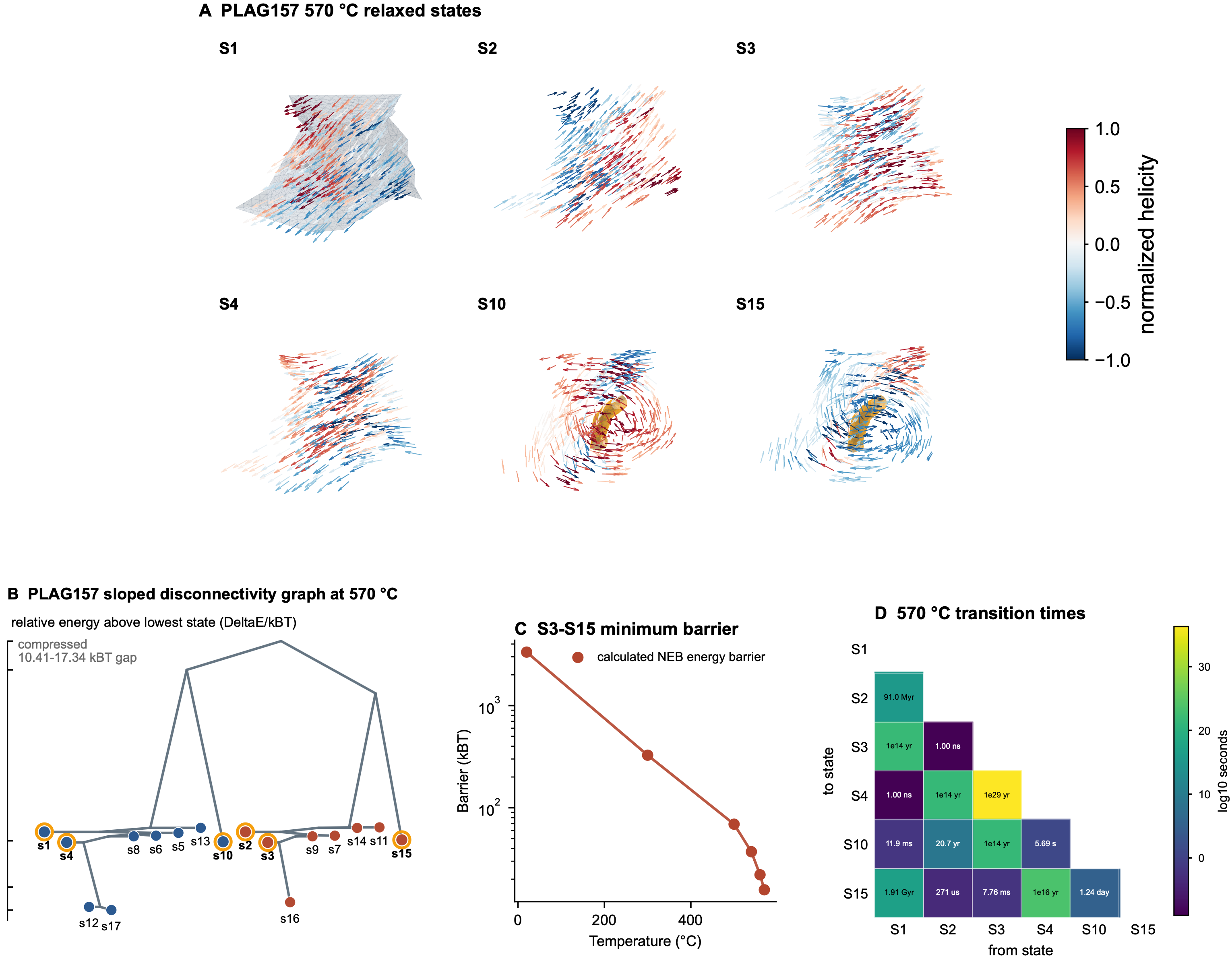
Micromagnetic application
Disconnectivity graphs

Slide 47

Micromagnetic application
Energy barrier vs. temperature

Slide 48

Micromagnetic application
transition matrix

Slide 49

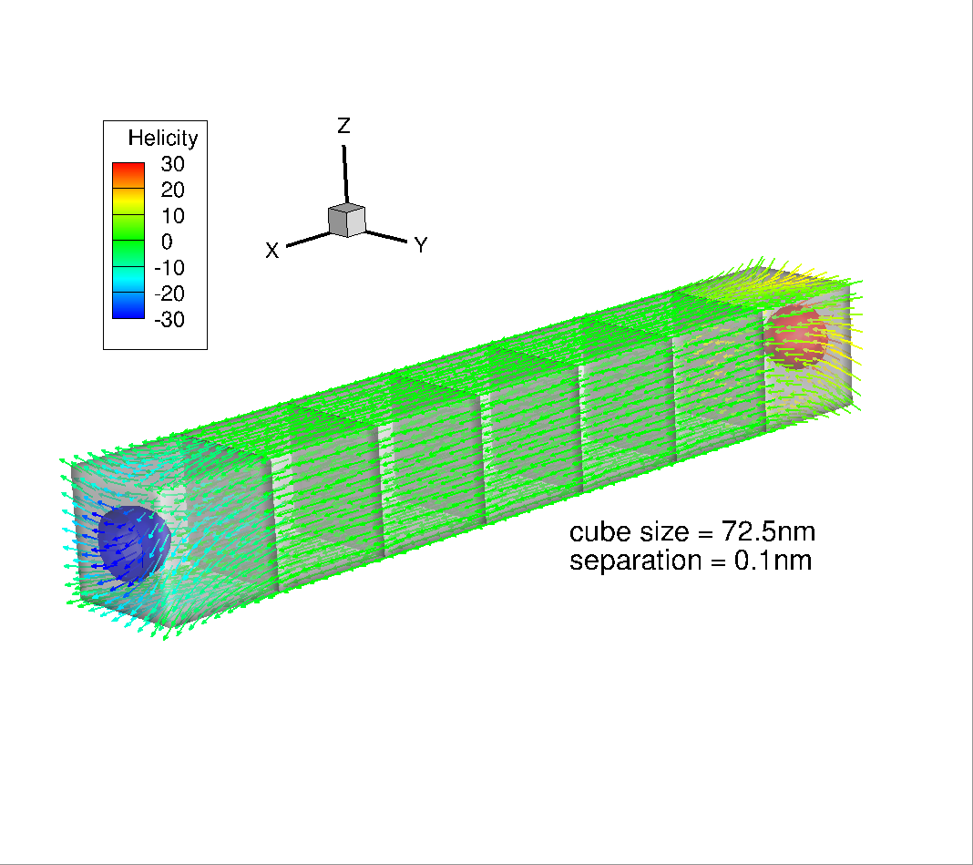
MERRILL – hands on

Example 5a….f

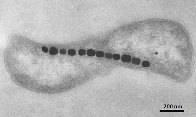
Source: Chen, Bazylinski & Lower (2010),
Nature Education Knowledge 3(10):30.

Modified slide from Wyn Williams

Slide 50

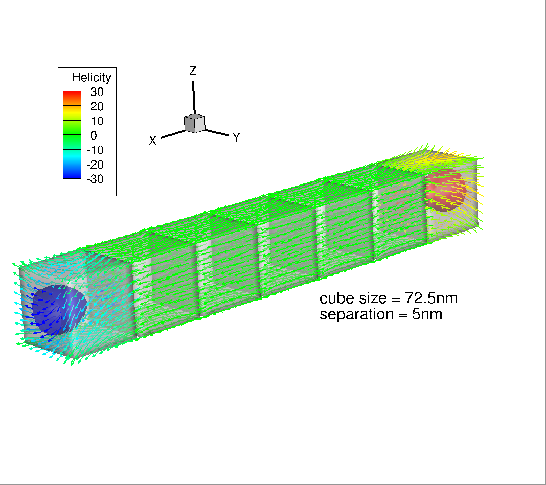
MERRILL – hands on

Example 5a….f

slide from Wyn Williams

Slide 51

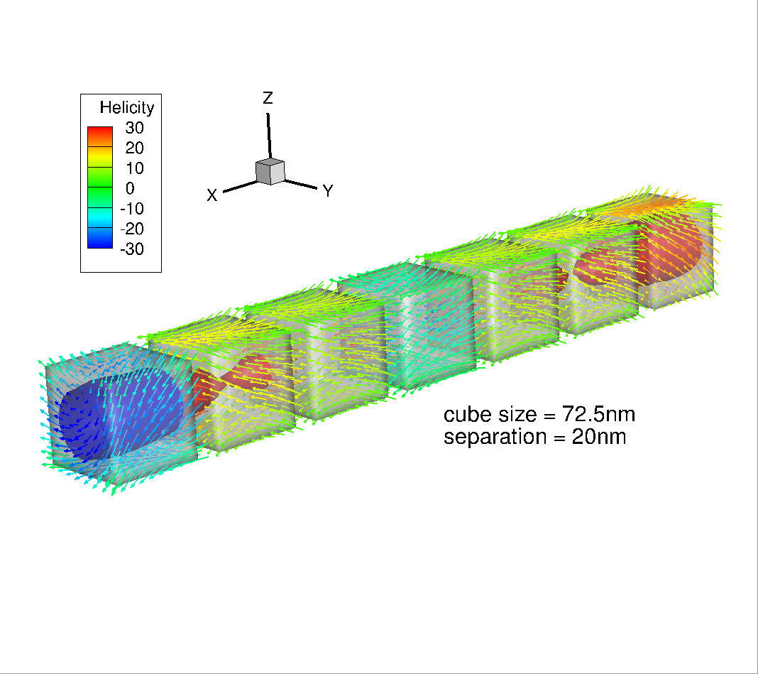
MERRILL – hands on

Example 5a….f

slide from Wyn Williams

Slide 52

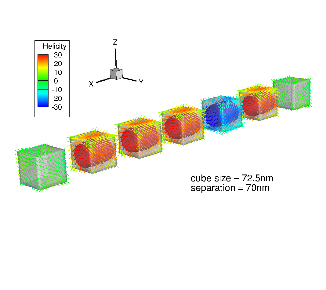
MERRILL – hands on

Example 5a….f

slide from Wyn Williams

Slide 53

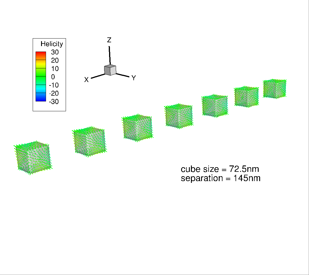
MERRILL – hands on

Example 5a….f

slide from Wyn Williams

Slide 54

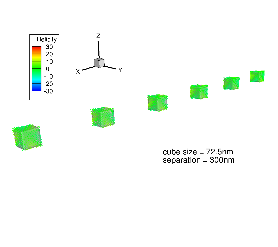
MERRILL – hands on

Example 5a….f

slide from Wyn Williams

Slide 55

MERRILL – hands on

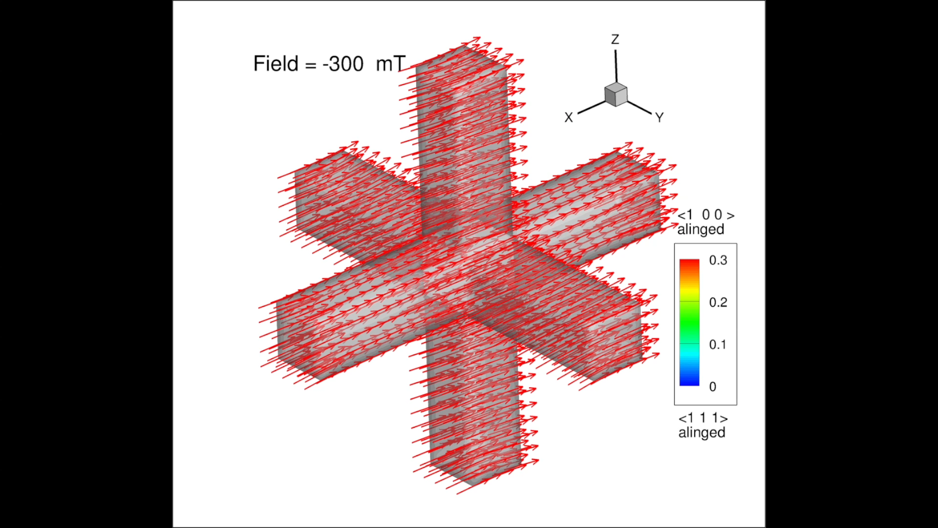
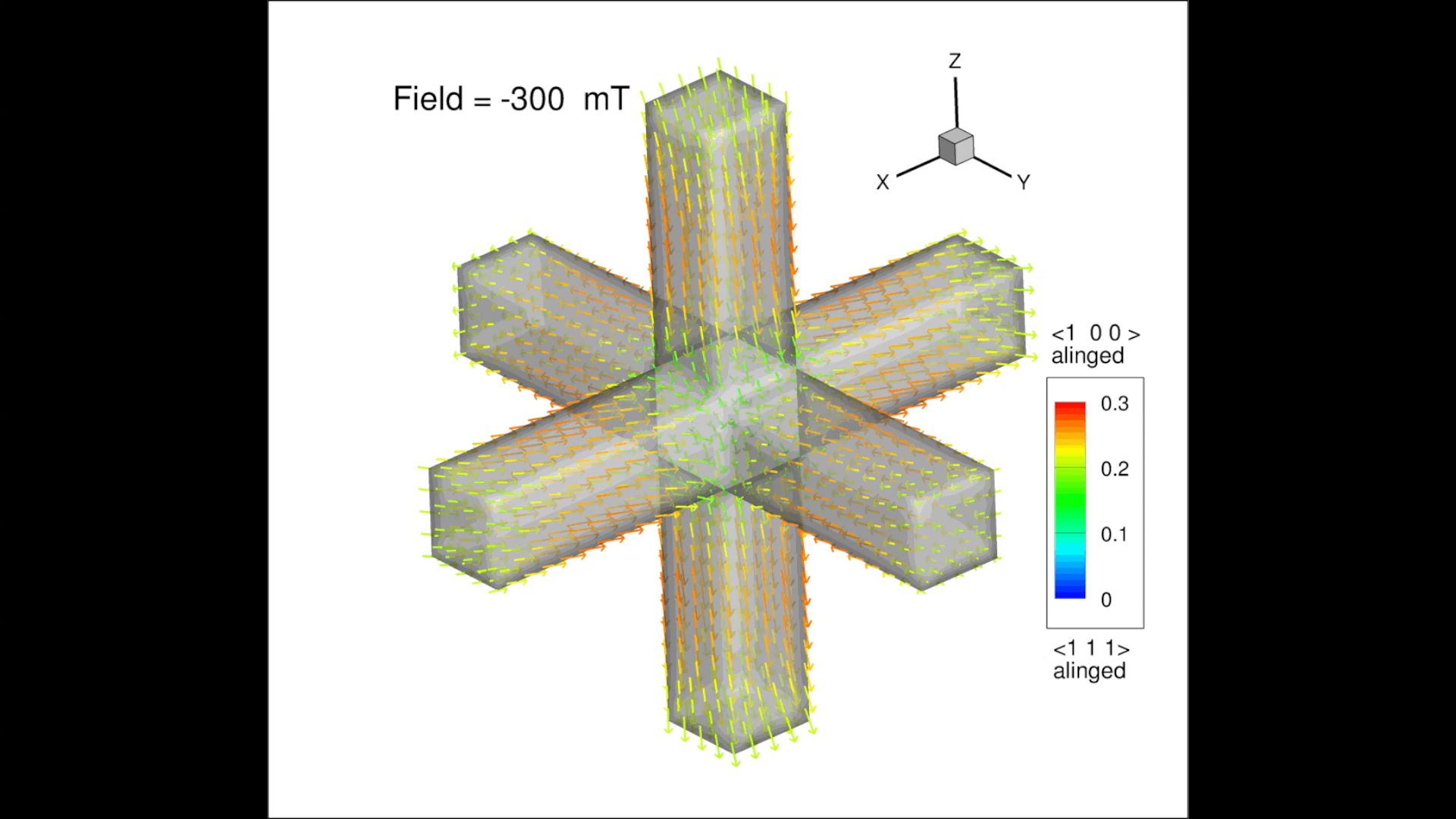
Field along ~ 1, 0, 0

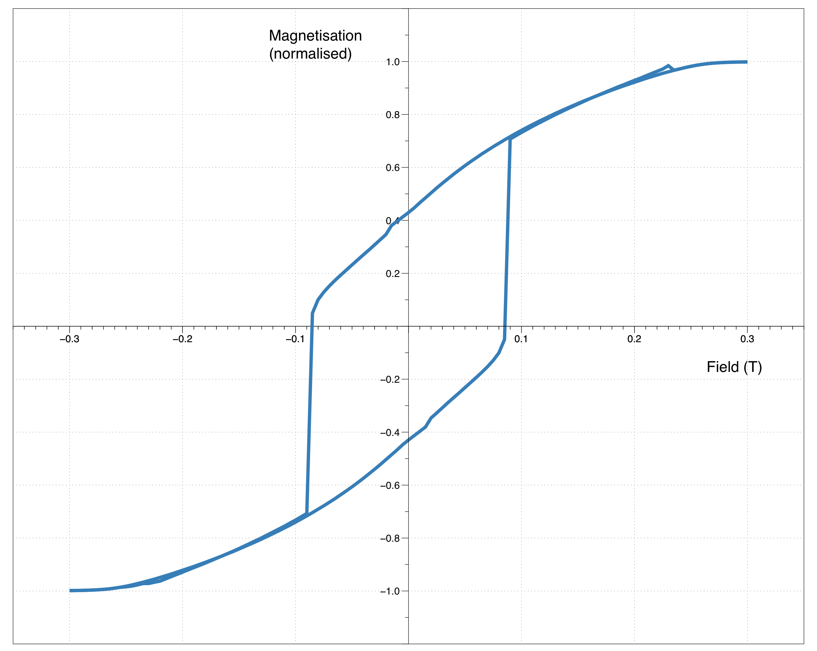
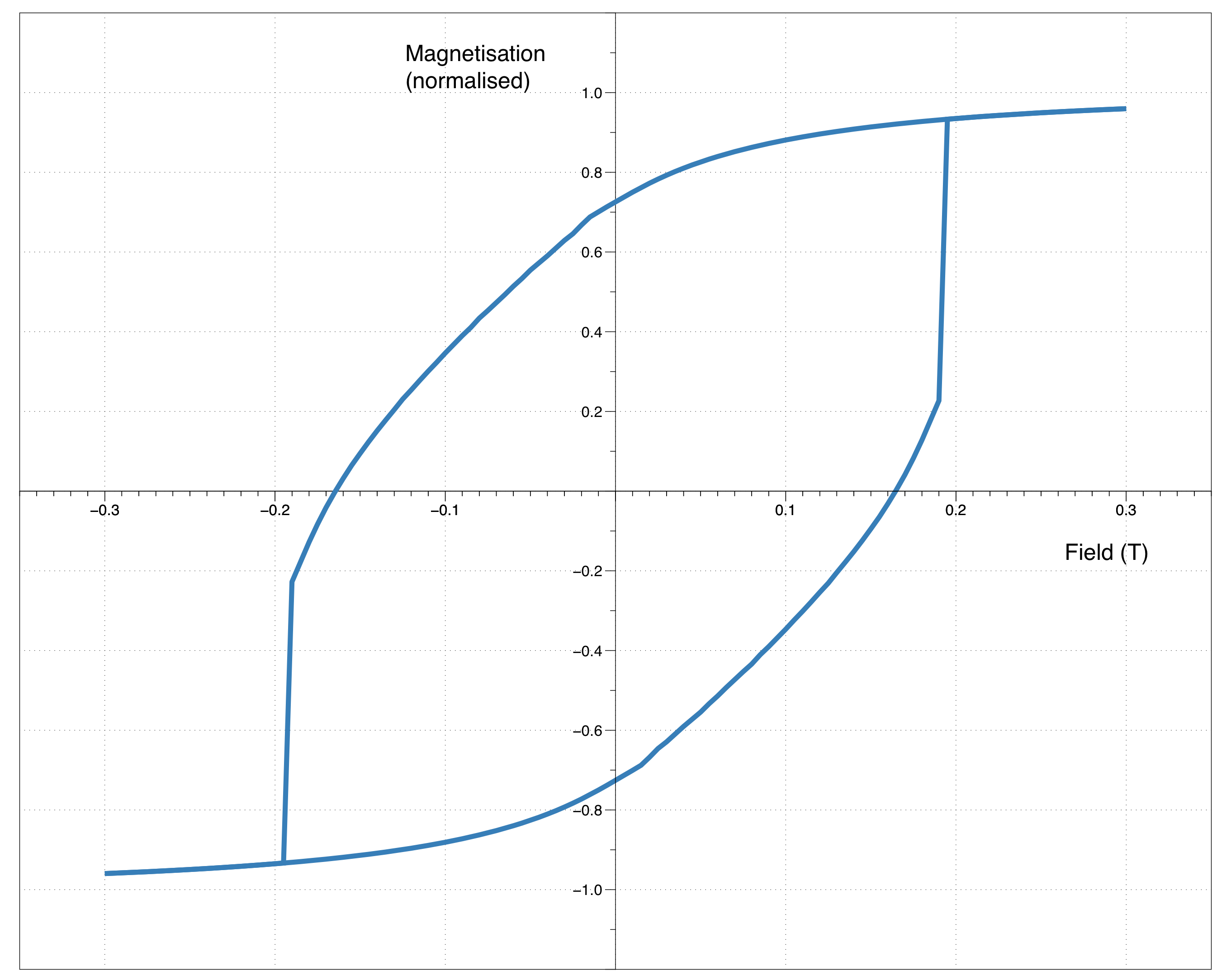
Field along ~ 1, 1, 1

slide from Wyn Williams

Slide 56

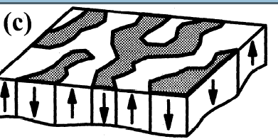
Micromagnetic modeling on an MD grain
1 µm magnetite cube

natural oxidized titanomagnetite (Krása et al., 2005)

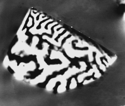
Pokhil and Moskowitz, 1997; Hurbert and Schäfer, 1998

+

+

+

+

+

+

-

-

-

-

-

Inside one domain wall

Inside one domain wall
Where it sits in the grain—and the nearly ideal Bloch-like rotation across it

Slide 57

Stray field modeling

Flower–vortex stray-field comparison

Flux closure weakens the stray field
A vortex lowers demagnetizing energy by accepting more exchange energy

Slide 58

Caveats

•Micromagnetic modeling can at best approximate reality

•Our computation and storage power do not allow modeling ensembles in a real bulk sample

•Quality of the initial micromagnetic mesh can dictate results